Suppose I’m thinking of a path between two complex numbers  and
and  , and I have a holomorphic function
  that I want you to integrate on the path. The problem is, I’m obnoxious, and I didn’t tell you what the path was. Can you do it?
The short answer is unfortunately no. The slightly longer answer is: it depends on the open set  . If has no holes, then you can do it. Sometimes, you can even if does have holes, but that’s not what we’re going to worry about. The claim is that if I can continuously morph one path
  into another path
  , then
Such a “continuous morphing” is called a homotopy. Maybe you can see, roughly speaking, how a hole could be an obstruction to morphing one path into another. The intuition is, if you tie down two ends of a string, and you stick a big “pole” in the ground. You can’t get the string to go around the other side of the pole (without lifting it off the ground).
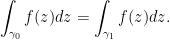
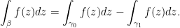
Here’s another way to look at it. Suppose I first integrate over the curve , and then I integrate over the curve , but I do it backwards. The result would be the difference between the two integrals. If  is the curve given by and then backwards, then
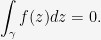
I’d like to show that this integral is zero. One way to do this would be to show that if I integrate over any loop which is homotopic (can be shrunk down) to a point, then the integral must be zero.
Indeed these two things are equivalent, but I’m not going to prove either. To avoid some messy details, and sweep some others under the rug, I’m going to prove a result that is slightly weaker, though I hope strong enough to give you the right idea. The details I’m leaving out aren’t complex analysis. They’re topology, and in my opinion, boring. I’ll prove this weaker result, and then use the stronger one. If you’re interested, Ahlfors has a proof of the stronger result.
This weaker result is about loops which enclose a simply-connected region. That is, it’s the same result as I want to prove, but only for loops which are the boundary of some region.
Theorem 1 Let  be a simply-connected region contained in an open set
  , and
, and ![{\gamma:[0,1]\rightarrow\partial R}](https://s0.wp.com/latex.php?latex=%7B%5Cgamma%3A%5B0%2C1%5D%5Crightarrow%5Cpartial+R%7D&bg=f5f5f5&fg=000000&s=0&c=20201002) is a parameterization of the boundary, then for
is a parameterization of the boundary, then for  ,
,
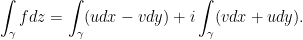
Proof: Let  , and let
  . Then we have the relation on 1-forms
  . As before, we’ll be using the notation
  as shorthand for
  . Now
. Now
From Green’s theorem (which we won’t prove because it is real analysis), we know that

and that

Of course, the Cauchy-Riemann equations tell us that  and
and  , so
, so
as desired. 
A discussion with some friends revealed that this is sort of a hack. I just swept the difficult part of the theoerm into Green’s theorem and then didn’t both to prove it. I know. But I like it anyway, and the reason I like it is because I had never seen the connection between the Cauchy-Riemann equations and the result of Green’s theorem. In some sense, one might say that complex analysis is the study of a very special class of functions that behave in remarkably nice ways with respect to Green’s theorem.
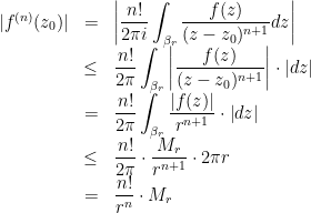
has at least one root in


 is bounded (i.e.,
  for some
  ), then
  is constant.
  . Recall that

 less than the radius of convergence of
  . Thus, for
  ,
,  can be bounded by arbitrarily small positive numbers. That is,
  for all
  , a constant.
  and
and  are holomorphic on all of
  is always between
  and
and  . You are correct for
  , but Liouville’s theorem doesn’t say anything about functions on
  . Indeed, if you plug in complex numbers, you’ll see that
  can be arbitrarily large. In fact, look at
  for
for  , and
, and  . If we have a circle
  of radius
  on
on  . We then argued that as
  ,
,  because
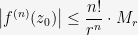
 , the result is exactly what we already used.
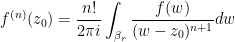
 , and any counterclockwise circle
  in
in  about
about  (or any loop homotopy equivalent to it in
  ),
),
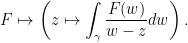
 , and it spits out another function depending on
  . That is,
 .
.  , and
, and  , as above. Then

 th derivative and evaluating at

 for
for  around
 , and I plugged in
  . By my definition,
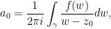
 . Pretty cool, huh?
 centered at
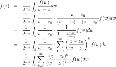
 will have the coefficient involving an integral that has
  in the denominator, just as
  does.
does.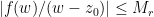 . Now we’re left with just
 , and
, and  . Thus, the entire fraction is less than 1 in absolute value. The sum over all
  of these is a geometric series which converges, and so the Weiersrass
  -test tells us that the the sum of the integrals is the integral of the sum. Thus

 students must be able to use at least
  as a pacman symbol with the
  inside the packman, and the
  in the mouth. They pronounced the symbol “
 . How what about the function
  ? It’s easy to check that it’s holomorphic on
  . You can do this by proving the applications of the multiplication rule and chain rule with one of the
 , such as the one to the left. The
 . A small circle going around
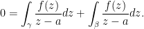
 , and
, and 

 given by
  . Then

 into the integral. To do so, we need to multiply it by
  because of the
  outside the integral. But we also need to divide by
  to
to 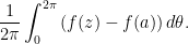
 get? I don’t have the slightest clue, but I can tell you that for the values
  attains its maximum on a compact set. Let
 and
and 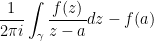
![{h:[a,b]\rightarrow{\mathbb C}}](https://s0.wp.com/latex.php?latex=%7Bh%3A%5Ba%2Cb%5D%5Crightarrow%7B%5Cmathbb+C%7D%7D&bg=ffffff&fg=000000&s=0&c=20201002) , then we will say that
, then we will say that  is integrable if
  and
and  are both integrable. For the pedantic, here I suppose I mean Riemann integrable. Anyway, if so, then we can define
![{\gamma:[a,b]\rightarrow{\mathbb C}}](https://s0.wp.com/latex.php?latex=%7B%5Cgamma%3A%5Ba%2Cb%5D%5Crightarrow%7B%5Cmathbb+C%7D%7D&bg=ffffff&fg=000000&s=0&c=20201002) is a path, and
is a path, and 
 . They’re certainly defined similarly. Anyway, let’s do an example. If
  for
for ![{t\in[0,2\pi]}](https://s0.wp.com/latex.php?latex=%7Bt%5Cin%5B0%2C2%5Cpi%5D%7D&bg=ffffff&fg=000000&s=0&c=20201002) , then
, then 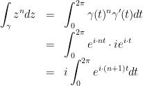
 , we have
  . Otherwise, the integral is
 is a reparameterization of
 . We’ll have
 ![{\beta:[a,b]\rightarrow{\mathbb C}}](https://s0.wp.com/latex.php?latex=%7B%5Cbeta%3A%5Ba%2Cb%5D%5Crightarrow%7B%5Cmathbb+C%7D%7D&bg=ffffff&fg=000000&s=0&c=20201002) ,
, ![{\gamma:[c,d]\rightarrow{\mathbb C}}](https://s0.wp.com/latex.php?latex=%7B%5Cgamma%3A%5Bc%2Cd%5D%5Crightarrow%7B%5Cmathbb+C%7D%7D&bg=ffffff&fg=000000&s=0&c=20201002) , and
, and ![{\phi:[a,b]\rightarrow[c,d]}](https://s0.wp.com/latex.php?latex=%7B%5Cphi%3A%5Ba%2Cb%5D%5Crightarrow%5Bc%2Cd%5D%7D&bg=ffffff&fg=000000&s=0&c=20201002) , all continuous. Then
, all continuous. Then 
 -substitution”
  , so
, so  , we get
 is also analytic, and with the same radius of convergence. Of course, it suffices to show power series; analytic functions being a bunch of “patched together” power series.
 for
for  be a power series centered at
  is also a power series, and has radius of convergence
 . It would be nice to show that
  . This comes down to showing that I can move the differential operator
  across the limit, so that
 uniformly, then I can. This is a standard theorem from analysis that I won’t prove. If you like, it’s theorem 7.17 in Baby Rudin. In general,
  need not be uniform, but on any ball with radius smaller than it’s radius of convergence, the limit is uniform. This is the same trick that we used yesterday to show that
 . Clearly this converges if and only if
  in
in  , so the radius of convergence is given by
![\displaystyle \left(\limsup_{n\rightarrow\infty}\sqrt[n]{n\cdot|a_n|}\right)^{-1}=\frac1{\displaystyle\lim_{n\rightarrow\infty}\sqrt[n]n}\cdot\left(\limsup_{n\rightarrow\infty}\sqrt[n]{|a_n|}\right)^{-1}=1\cdot R.](https://s0.wp.com/latex.php?latex=%5Cdisplaystyle+%5Cleft%28%5Climsup_%7Bn%5Crightarrow%5Cinfty%7D%5Csqrt%5Bn%5D%7Bn%5Ccdot%7Ca_n%7C%7D%5Cright%29%5E%7B-1%7D%3D%5Cfrac1%7B%5Cdisplaystyle%5Clim_%7Bn%5Crightarrow%5Cinfty%7D%5Csqrt%5Bn%5Dn%7D%5Ccdot%5Cleft%28%5Climsup_%7Bn%5Crightarrow%5Cinfty%7D%5Csqrt%5Bn%5D%7B%7Ca_n%7C%7D%5Cright%29%5E%7B-1%7D%3D1%5Ccdot+R.&bg=ffffff&fg=000000&s=0&c=20201002)
 . Locally,
  . Then
  . Also,
  analytic, so
  . In general,
  is analaytic, and so
  . Thus,